 Posted on January 28, 2025 by Nate_007 Reads:
 Introduction
Welcome to my post comparing moving average calculations in MATLAB vs Python (Pandas & Matplotlib). Calculating moving averages is an important part of stock market analysis, economics, weather forecasting, and signal processing. Most universities these days teach MATLAB as part of any mathematical, science or engineerings degree but licensing can be rather expensive and if you can't afford paying the subscription MATLAB is not a viable option post degree. Cue Python! Python is an high level open source object-oriented programming language thats free to use and distribute, it also have a large community of users online and a vast repository of libraries to meet you everyday programming needs. For data analytics Python is a valuable tool to have in your toolkit.
Moving Average MATLAB
Step 1: Get stock dataset
for this comparison i chose to use Microsofts share price data obtained from Nasdaq at https://www.nasdaq.com/market-activity/stocks/msft/historical then i download the 5y data set.
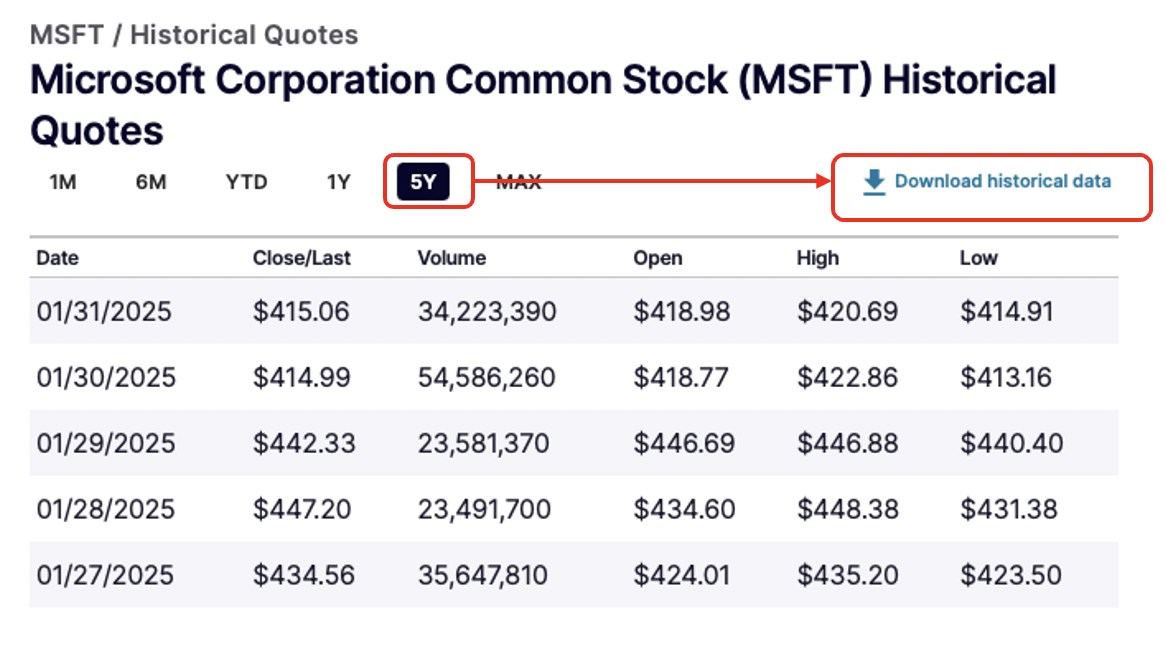
Step 2: Import data into MATLAB
once you have the data set then you can open MATLAB to import the data. the data can be imported using the following code
% Set up the Import Options and import the data
imp_opts = delimitedTextImportOptions("NumVariables", 6);

% Specify range and delimiter
imp_opts.DataLines = [2, Inf];
imp_opts.Delimiter = ",";

% Specify column names and types
imp_opts.VariableNames = ["Date", "Last_Close", "Volume", "Open", "High", "Low"];
imp_opts.VariableTypes = ["datetime", "double", "double", "double", "double", "double"];

% Specify file level properties
imp_opts.ExtraColumnsRule = "ignore";
imp_opts.EmptyLineRule = "read";

% Specify variable properties
imp_opts = setvaropts(imp_opts, "Date", "InputFormat", "MM/dd/yyyy");
imp_opts = setvaropts(imp_opts, ["Last_Close", "Open", "High", "Low"], "TrimNonNumeric", true);
imp_opts = setvaropts(imp_opts, ["Last_Close", "Open", "High", "Low"], "ThousandsSeparator", ",");

% Import the data
data = readtimetable("/Users/THELAB/Documents/Uni/HIT137/pandas_demos/HistoricalData_1738382886040.csv", imp_opts, "RowTimes", "Date");

% Clear temporary variables
clear imp_opts
Step 3: Create moving average function
To apply moving average in MATLAB without having access to the financial toolbox, a function will need to be developed to perform the calculation
function result = moving_average(data, window_size)
    % Check if the input is a timetable
    if istimetable(data)
        dataValues = data.Variables;
    else
        dataValues = data;
    end

    % Ensure the data is a row vector
    if iscolumn(dataValues)
        dataValues = dataValues';
    end

    % Validate the window size
    if window_size <= 0 || window_size > length(dataValues)
        error('Invalid window size. It should be a positive integer less than or equal to the length of the data.');
    end

    % Preallocate the result array with NaN for positions where the window cannot be applied
    result = NaN(1, length(dataValues));

    % Compute the moving average
    half_window = floor(window_size / 2);
    for i = half_window + 1:length(dataValues) - half_window
        result(i) = mean(dataValues(i - half_window:i + half_window));
    end

    % If the input was a timetable, return a timetable
    if istimetable(data)
        result = array2timetable(result', 'RowTimes', data.Properties.RowTimes);
    end
end
Step 4: Apply filter and calculate
Before the data can be plotted it needs to be reduce to the range that is going to be analysed and then the moving average function applied to create the moving average array so that the raw data can be overlaid with the average
% Filter date range to 2024
dt2024 = data(timerange('2024-01-01', '2024-12-31'), :);


% Create Last_Close array and apply 7 day moving average calculation
close24 = dt2024(:,"Last_Close");
maShort = moving_average(close24,7);
Step 5: Plot result
To plot the result, it will require plotting two plot using hold on and setting some custom tick arrangements to display the data correctly
figure;
plot(dt2024.Date, dt2024.Last_Close, 'LineWidth', 2,'DisplayName', 'Last Close');
xlabel('Date');
title ("Closing Price for 2024")
% Define the number of x-ticks (12 months)
num_xticks = 13;
xtick_positions = linspace(min(dt2024.Date), max(dt2024.Date), num_xticks);
xticks(xtick_positions);

% Set custom x-tick labels
x_labels = {'Jan', 'Feb', 'Mar', 'Apr', 'May', 'Jun', 'Jul', 'Aug', 'Sep', 'Oct', 'Nov', 'Dec', 'Jan'};
xticklabels(x_labels);

% Plot the moving average
hold on;
plot(dt2024.Date, maShort.Var1, 'LineWidth',2 ,'DisplayName', '7-day Moving Average', 'Color', 'r');
legend;
ylabel("Closing Price ($)");
hold off;
Finally we run the code and get the following output!
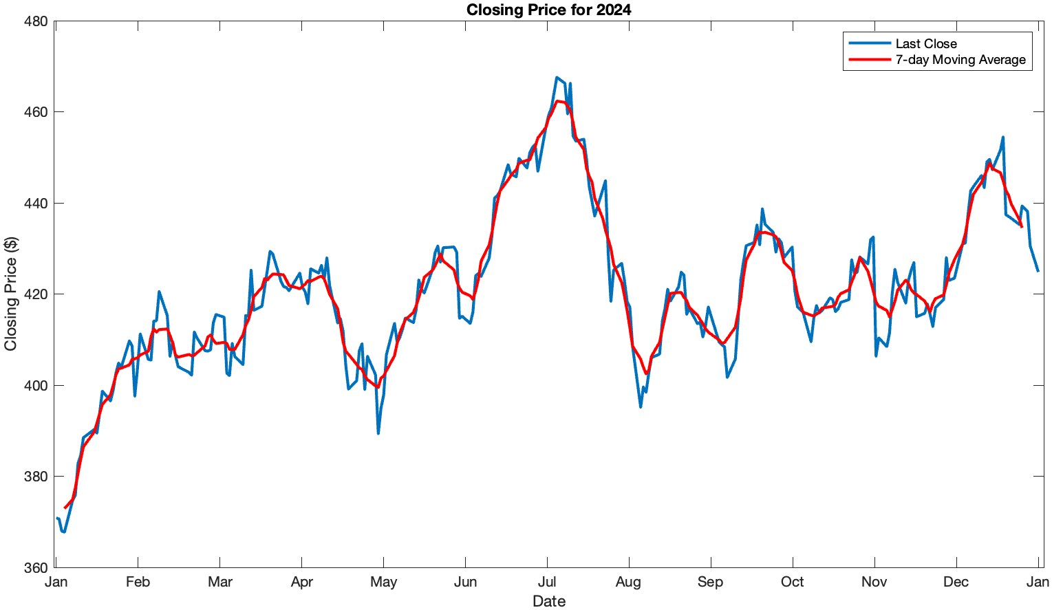
Now let recreate this using Python..
Moving Average Python (Pandas & Matplotlib)
Step 1: Install required libraries & import the data
If you do not have pandas or matplotlib you'll have to install the libraries first
pip install pandas matplotlibonce the libraries are install import the data and apply conversions to remove unwanted components of the data to make it easier for it be interpreted
import pandas as pd
import matplotlib.pyplot as plt
import matplotlib.dates as mdates

pd.options.mode.copy_on_write = True

data = pd.read_csv('/Users/THELAB/Documents/Uni/HIT137/pandas_demos/HistoricalData_1738382886040.csv')

# Parse the 'Date' column to datetime
data['Date'] = pd.to_datetime(data['Date'])

# Remove the dollar signs and convert columns to numeric
data['Close/Last'] = data['Close/Last'].str.replace('$', '').astype(float)
data['Open'] = data['Open'].str.replace('$', '').astype(float)
data['High'] = data['High'].str.replace('$', '').astype(float)
data['Low'] = data['Low'].str.replace('$', '').astype(float)

# Set the 'Date' column as the index
data.set_index('Date', inplace=True)
Step 2: Filter and apply moving average
In the python method of applying moving average we don't need to create a function as the pandas function rolling combined with mean {rolling().mean()} does the same thing so we can use this combo instead which will greatly reduce the code required
# Filter data for the year 2024
data_2024 = data.loc['2024']

# Calculate the moving average (e.g., 30-day moving average)
data_2024.loc[:,'Moving_Avg'] = data_2024['Close/Last'].rolling(window=7,center=True).mean()
Step 3: Plot result
For the plotting the matplotlib library is use to create subplots of each of the arrays creating the overlay
# Plot the closing price for 2024
fig, ax = plt.subplots()
data_2024['Close/Last'].plot(kind='line', ax=ax, title='Closing Price for 2024')
ax.set_xlabel('Month')
ax.set_ylabel('Closing Price ($)')

# Plot the moving average
data_2024['Moving_Avg'].plot(kind='line', ax=ax, color='red', label='7-Day Moving Average')

# Format the x-axis to show each month
ax.xaxis.set_major_locator(mdates.MonthLocator())
ax.xaxis.set_major_formatter(mdates.DateFormatter('%b'))

# Ensure the x-axis covers the full year
ax.set_xlim([pd.Timestamp('2024-01-01'), pd.Timestamp('2024-12-31')])

plt.legend()
plt.show()
Finally run the code to view the plotted output!
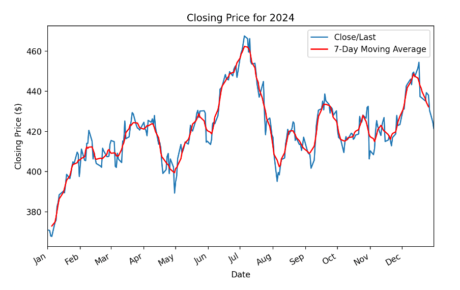
Conclusion
As you can see from the results of both plots they are nearly identical. some might argue that MATLAB will calculate it faster and have better performance but it does come with the price tag, if you are looking to run a series of calculation where speed isn't an issue then Python is an excellent tool thats free to use.